TL;DR — Deconvolution in Microscopy: Sharper Images, Better Data. Deconvolution removes blur in microscopy by reversing the point spread function, yielding sharper images and more reliable measurements. From Richardson–Lucy origins to modern tools like AutoQuant, it underpins accurate 3D imaging across biology, medicine, and materials science.
 After
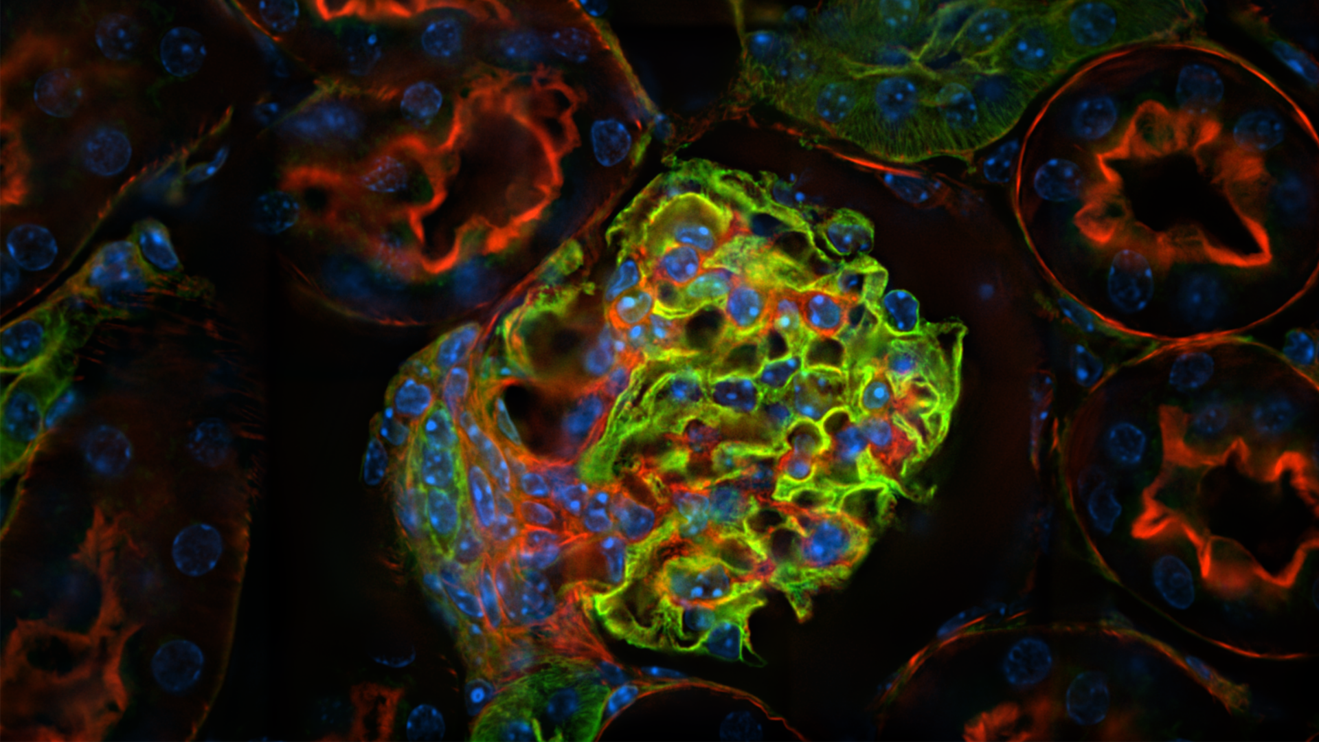
After
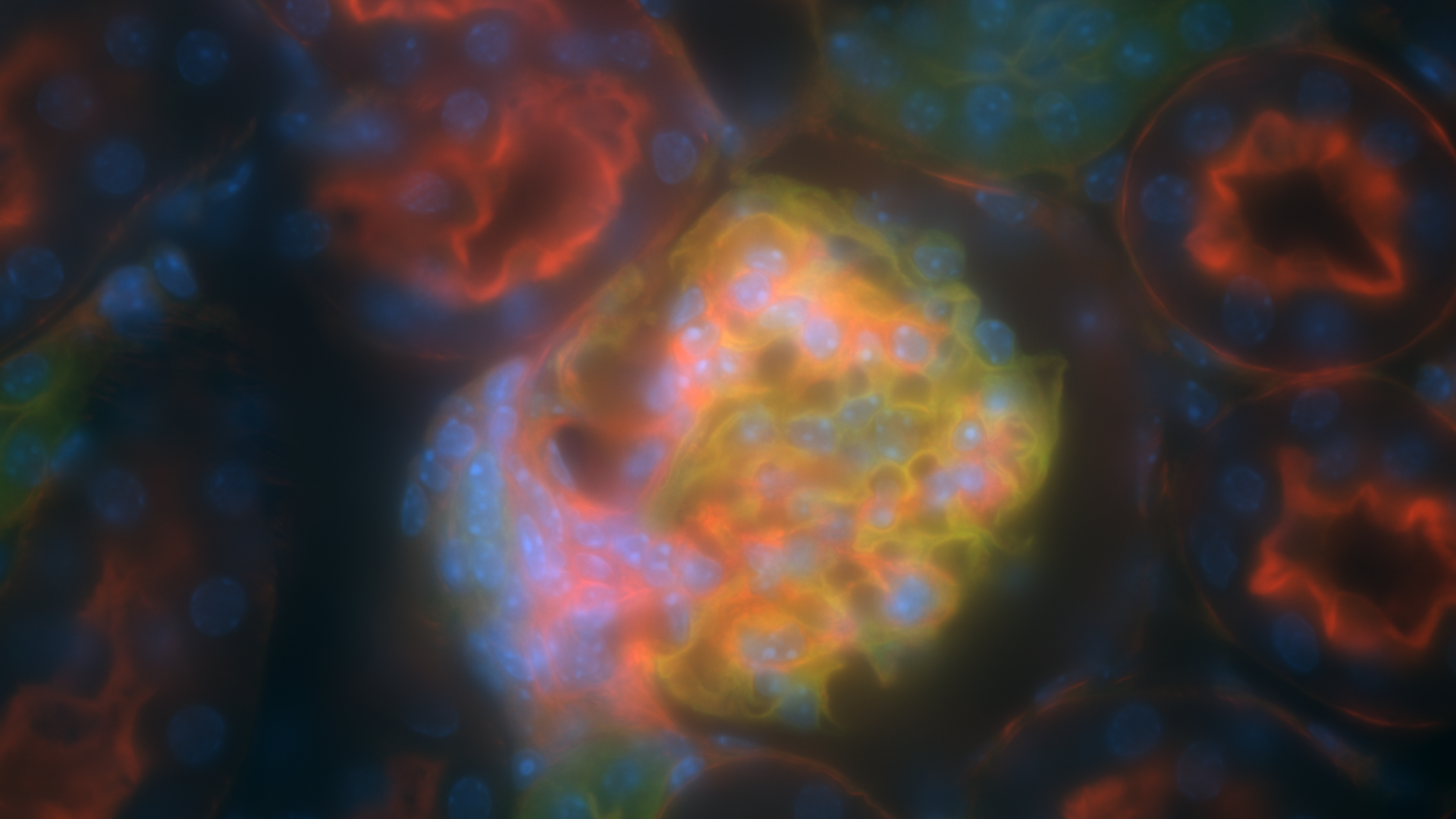 Before
Figure 1. Before and after image.
Seeing Through the Blur
Microscopy has transformed how we explore biology, medicine, and materials science. Yet, no image captured through a microscope is ever a perfect reflection of the sample. Light spreads, scatters, and interacts with the optics, creating blur and noise that obscure critical details. Deconvolution is a computational technique designed to reverse this blur, restoring clarity and revealing structures that would otherwise remain hidden.
This beginner’s guide provides a high-level overview of deconvolution, its methods, and why it matters, all while pointing readers to deeper technical resources and examples from published studies.
What is Deconvolution in Microscopy?
At its core, deconvolution is a computational method that reverses the blurring effects of a microscope by mathematically reassigning photons back to their most likely points of origin. This process depends on the Point Spread Function (PSF), which is a model of how a single point of light spreads when imaged through the optical system. In practice:
Observed image = True sample × PSF + Noise
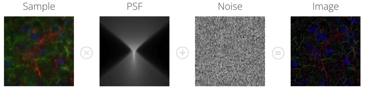
Figure 2. How an image is created.
By estimating and iteratively correcting the PSF, deconvolution sharpens images, increases contrast, and enables more accurate measurement of biological and material structures.
The theoretical foundation for this approach was strengthened by Streibl (1984), who described how axial (depth) information transfers through an imaging system via the PSF and Optical Transfer Function (OTF). His work explained why depth-dependent blur occurs and why measured versus theoretical PSFs can produce different outcomes. This insight laid the groundwork for modern deconvolution techniques by showing that accurately modeling the PSF is essential for reliable 3D image reconstruction.
Where deconvolution can make the biggest impact:
- Cell biology (organelle visualization)
- Neuroscience (synaptic resolution)
- Digital pathology (tissue clarity)
- Materials science (grain boundaries, defects)
History of Deconvolution
The origins of deconvolution trace back to astronomy, where Richardson (1972) and Lucy (1974) introduced an iterative statistical method to restore blurred telescope images. Their approach, now known as the Richardson–Lucy algorithm, became the foundation for later applications in microscopy.
By the early 1980s, Agard and Sedat (1983) demonstrated that computational restoration could dramatically improve biological imaging, reconstructing polytene chromosomes in three dimensions. This work established the idea of 'deconvolution microscopy' and influenced decades of imaging research.
Why Deconvolution Matters
Blurred images are more than just an aesthetic problem, because they can mislead quantitative analysis. For instance, small organelles may appear merged, or signal intensity may be underestimated, leading to faulty conclusions.
As discussed in our post on the Frustrating Realities of Image Analysis, researchers often struggle with noise, artifacts, and data volume. Deconvolution addresses these frustrations directly by extracting the most reliable information from each dataset, helping ensure that downstream analysis reflects biological or structural reality.
Deconvolution Methods in Microscopy: Fixed PSF and Iterative Approaches
The accuracy of deconvolution depends heavily on the point spread function (PSF). If the PSF does not reflect how light truly behaves in the microscope, the reconstruction will be unreliable. Model et al. (2011) demonstrated this clearly: spherical aberrations from refractive-index mismatches can bend and blur reconstructions, making structures appear distorted unless proper PSF measurement and aberration correction are applied.
Practical validation is equally important. Lee (2014) calibrated wide-field deconvolution in AutoQuant using fluorescent bead stacks and confirmed that the algorithms preserved relative quantitative intensity relationships in 3D data. In Lee’s words, “the deconvolution algorithms in AutoQuant X3 preserve relative quantitative intensity data.” This shows that well-designed tools not only sharpen images but also maintain trustworthy measurements.
Together, these examples highlight a core principle: effective deconvolution is as much about accuracy and reproducibility as it is about visual clarity.
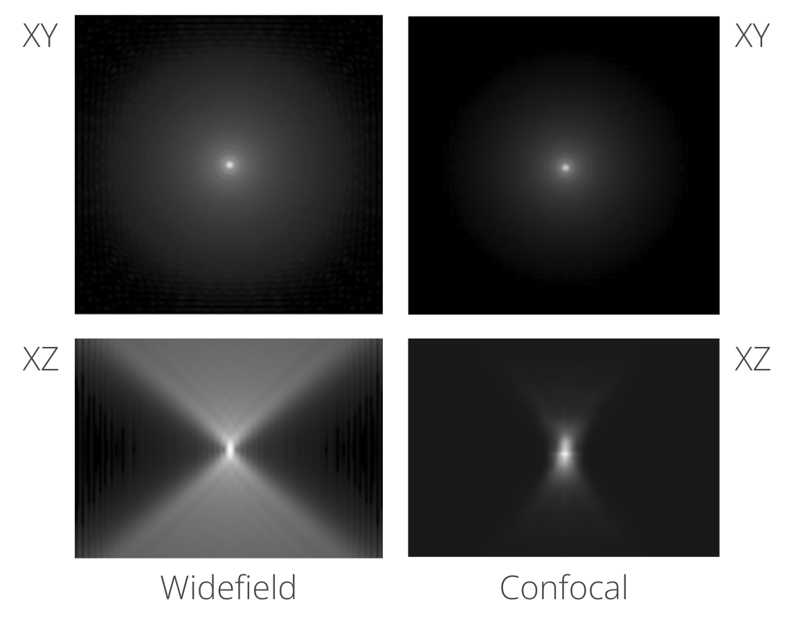
Figure 3. Examples of the PSF in XY and XZ for both Widefield and Confocal microscopes.
Fixed PSF Approaches
In many practical workflows, deconvolution uses a fixed PSF (either measured or theoretical). You collect or compute one PSF, then use it through the entire deconvolution process.
- Measured PSF — imaging sub-resolution beads under the same optical conditions gives an empirical PSF that captures aberrations, misalignments, and depth-dependent distortions.
- Theoretical PSF — computed from known optical parameters (NA, refractive index, immersion medium, emission wavelength, coverslip thickness). It’s more convenient and reproducible, though it may miss sample-specific aberrations if not accounted for.
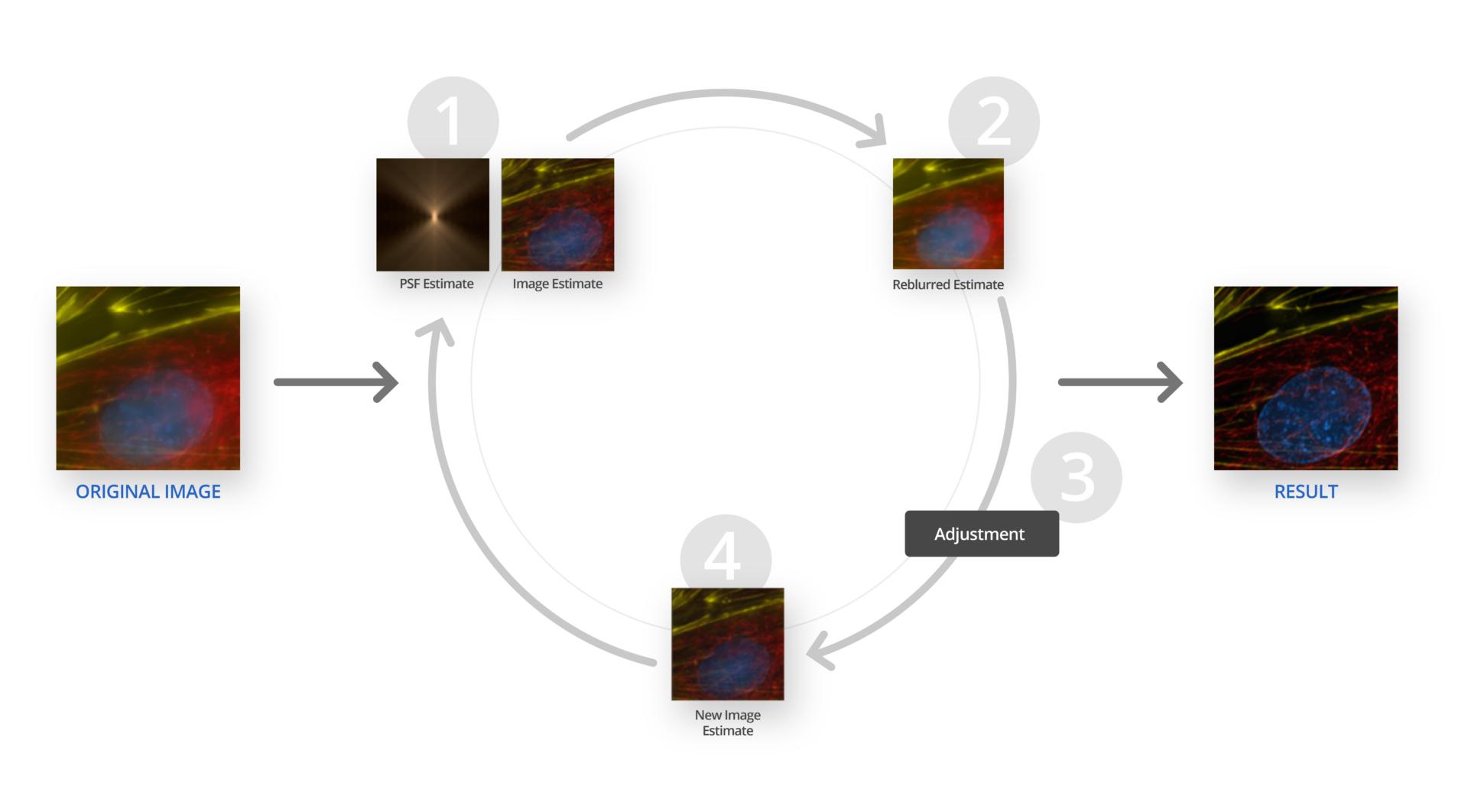
Figure 4. Diagram of the deconvolution iterative refinement cycle.
Iterative Refinement & Convergence Behavior
Most modern deconvolution algorithms work through iteration, meaning they make an initial guess of the true image, compare it to the blurred data, and then repeatedly adjust the guess. With each cycle, the estimate becomes sharper and closer to the real structure, while trying not to amplify noise.
The way these algorithms “converge,” or settle on a final solution, is critical. In their classic paper, “Fast maximum-likelihood image-restoration algorithms for three-dimensional fluorescence microscopy” (Markham & Conchello, 2001), the authors compared several strategies, including expectation-maximization (EM), conjugate gradient methods, and divergence-based approaches. They found that some of these optimizations reached accurate solutions much faster, showing that not all iterative methods are equal when speed and stability matter.
To further stabilize results, researchers often use regularization, which sets mathematical safeguards that prevent the algorithm from overfitting to random noise. Combined with GPU acceleration, which dramatically reduces computation times, these strategies make it practical to run deconvolution on today’s large 3D datasets. The result is an approach that not only enhances images but does so reliably and efficiently, turning raw microscope data into information scientists can trust.
Tips and Common Pitfalls in Microscopy Deconvolution
For readers seeking further guidance, Wallace, Schaefer & Swedlow (2001) remains a classic reference, which remains a practical guide for setting iterations, recognizing artifacts, and validating deconvolution results.
Deconvolution is powerful, but misapplication can lead to misleading results.
Here are tips and common pitfalls to watch:
- Start with conservative iteration counts. Too few leave blur; too many may amplify noise or generate ringing.
- Validate with controls. Use fluorescent bead or known-geometry samples to check whether deconvolution is restoring known features rather than inventing new ones.
- Match optical conditions. If using measured PSF, match objective, immersion medium, refractive index, and coverslip thickness.
- Be cautious with tiling / stitching. Large volumes often get processed in subvolumes; ensure overlap and smoothing to avoid seam boundaries.
- Monitor dynamic range shifts. Because much background blur is reassigned, mid-level or faint areas can darken; adjust display scaling or contrast accordingly.
Comparison of Deconvolution Approaches
| Approach | PSF Source | Strengths | Risks / Limitations | Best Use Case |
|---|---|---|---|---|
|
Fixed PSF — Measured |
Empirically captured beads |
Captures real aberrations and system idiosyncrasies |
Acquiring good beads may be laborious; sensitive to small misalignments |
Precision experiments, deep imaging |
|
Fixed PSF — Theoretical |
Modeled from optics |
Convenient, reproducible, flexible |
May miss sample-specific aberrations or depth effects |
Routine deconvolution workflows |
Table 1. Comparison of Measured and Theoretical PSF strengths and limitations.
Final Thoughts
Deconvolution has evolved from a niche, computational experiment into a standard part of the microscopist’s toolkit. By correcting the blur introduced by the optics, it transforms raw images into clearer, more accurate representations of biological and material structures. Just as importantly, it safeguards quantitative integrity, ensuring that what looks sharper is also truer to the sample.
Today, many research labs rely on integrated platforms that make these advanced methods accessible without requiring deep programming or optics expertise. For example, life science imaging software such as Image-Pro AI For Life Science incorporates validated deconvolution tools directly into analysis workflows for fluorescence microscopy. This means researchers can move more confidently from image capture to measurement, focusing on discovery rather than troubleshooting algorithms.
Key Takeaways
- Deconvolution uses a fixed PSF plus iterative methods to reverse microscope-induced blur.
- It can make images sharper, increase contrast, and improve measurement reliability.
- Convergence behavior and regularization strategies (as studied in classical ML/EM deconvolution work) significantly affect performance.
- Validating results with controlled samples is crucial to avoid artifacts.
Frequently Asked Questions
A successful deconvolution should reveal sharper features without obvious artifacts such as halos, ringing, or seams. A good practice is to compare against control samples (e.g., fluorescent beads) and confirm that intensity trends remain consistent across the dataset.
There is no universal number. Too few iterations may leave residual blur; too many can introduce artifacts. Many workflows start with 10–15 iterations and adjust based on the data quality and algorithm used.
Confocal microscopy reduces out-of-focus blur optically by rejecting light outside the focal plane. Deconvolution, in contrast, is computational and can be applied to widefield, confocal, or even multiphoton data. In many cases, combining confocal imaging with deconvolution yields the best results.
Yes. By reassigning blurred light to its proper origin, deconvolution effectively reduces background and enhances contrast, which improves SNR. However, it does not create new signal and cannot recover information that was never captured in the raw data.
When applied correctly, deconvolution improves the accuracy of size, intensity, and positional measurements. Peer-reviewed studies have shown that while absolute intensity values may shift, relative trends remain preserved, which supports reliable quantification.
Not essential, but very helpful. For large 3D datasets, GPU-based deconvolution can reduce processing times from hours to minutes, making it practical for high-throughput workflows.
Not always. Theoretical PSFs work well for many imaging setups and are easy to generate. Measured PSFs are recommended for precision applications or when imaging conditions deviate from the ideal (e.g., depth-dependent aberrations).

Media Cybernetics
sales@mediacy.com
Related Links