If you follow the buzz around AI-powered image analysis, you’ve heard “CNN” tossed around more times than there are cat pictures on the internet. A Convolutional Neural Network is simply a neural network that tacks a clever, image-savvy “front end” onto the classic fully connected “back end,” letting the model tease out shapes, textures, and edges before it ever tries to name what it sees. That marriage of a front-end feature extractor plus a back-end classifier is why CNNs have become the workhorse of modern microscopy analysis — and why they’re worth understanding.
New to AI image analysis? Check out our Beginner’s Guide to AI-Powered Microscopy Image Analysis for a step-by-step walkthrough before diving deeper.
Why Images Challenge Algorithms
At first glance, image segmentation might seem straightforward: identify the shapes in a picture and draw boundaries around them. But real-world microscopy images are often single-channel gray scale, full of faint edges, overlapping cells, or wispy fibers. A single global threshold can’t cope with that chaos, so rule-based algorithms buckle.
If you’ve ever hit those pain points yourself, our candid blog on the Frustrating Realities of Image Analysis breaks down why they occur—and how modern AI tools can help. CNNs sidestep rigidity by learning from labeled examples instead of relying on fixed rules.
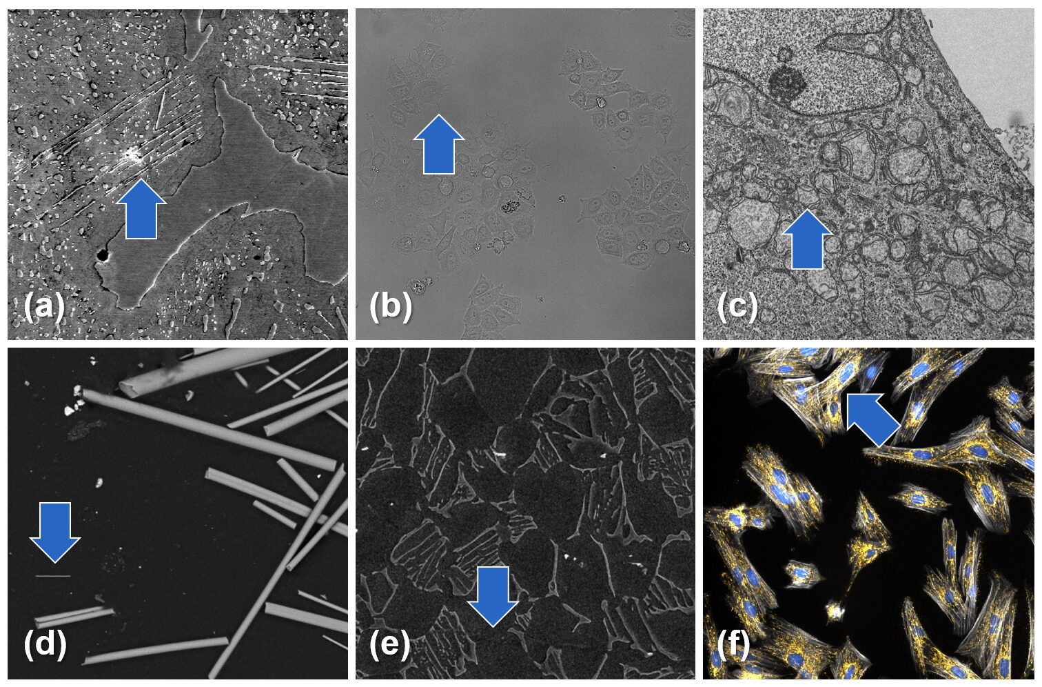
Figure 1. Example images showing common challenges such as (a) complex objects hard to separate from the background, (b) single-channel grayscale input, lacking color cues, (c) Multiple structures of similar size, shape, and intensity, (d) variability in size and morphology of target objects, (e) objects with low contrast or indistinct edges, and (f) touching objects with complex, interconnected shapes.
The Two-Stage Pipeline Inside Every CNN
| Stage | What Happens | Rough Ingredients |
|---|---|---|
|
Front-End: Feature Extractor |
Turns raw pixels into compact, informative feature maps |
Convolution → ReLU → Pooling (repeated) |
|
Back-End: Classifier Head |
Converts those maps into final labels |
One or two fully connected (dense) layers |
Table 1. Overview of the two core stages in a Convolutional Neural Network (CNN), summarizing their roles and operations.
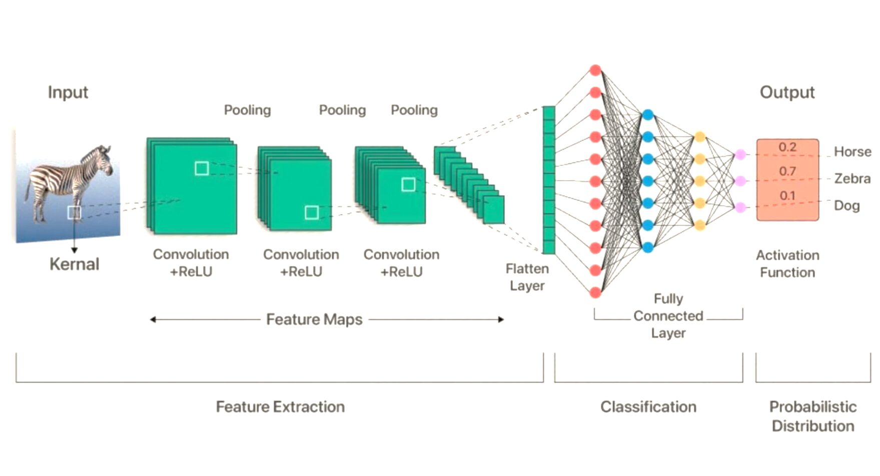
Figure 2. A left-to-right schematic illustrating the full journey of an image through a convolutional neural network (CNN).
1. Feature Extraction: A Crash Course
- Convolutional layers slide learnable filters (think 3 × 3 or 5 × 5 stencils) across small patches of the image. Each filter starts as random numbers but, during training, morphs into a detector for edges, corners, or textures. Because the same filter slides everywhere, the network shares weights—dramatically cutting parameters compared with connecting every pixel to every neuron.
- Activation functions—usually ReLU—follow each convolution. ReLU simply keeps positive values and zero negatives, adding a splash of needed non-linearity so stacked layers can model curves, blobs, or anything curvy in between.
- Pooling layers (max or average) shrink the feature maps. Imagine keeping the brightest pixel in every 2 × 2 block. This reduces memory, speeds computation, and gives the model a dose of translation tolerance—if your nucleus shifts a few pixels, the pooled signal hardly changes.
Layer by layer, the network graduates from “Hey, that’s an edge” to “That cluster looks suspiciously like a nucleus.” Early layers detect simple shapes; deeper ones capture entire cells.
Why does this matter? Feature extraction relieves the classifier from staring at 262,144 raw pixel values (for a 512 × 512 image) and hands it a neat bundle of maybe a few thousand high-level descriptors that scream “nucleus here, background there.”
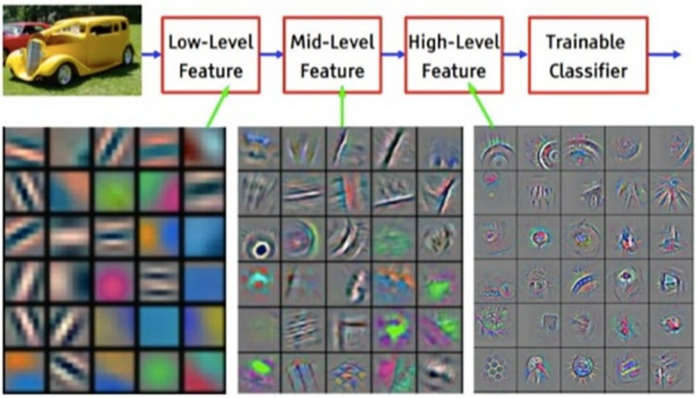
Figure 3. CNN hierarchy. A yellow vintage car enters the network, early layers detect edges and color blobs, mid-layers combine them into curves and motifs, and deep layers fire on wheels and other parts, feeding a classifier that outputs the car label. Ex. taken from Yann LeCun, 2015.

Figure 4. Max vs. average pooling. With a 2 × 2, stride-2 window, max pooling keeps each block’s peak (7) while average pooling outputs its mean (3). Source.
2. Classification: (a.k.a. The Fully Connected Finale)
After the image has been boiled down to tidy vectors, dense layers take over.
- Flattening unwraps the 3-D stack of feature maps into a 1-D vector—picture unrolling a sleeping bag.
- Fully connected (dense) layers link every input value to every neuron, each connection holding a trainable weight plus a bias.
- Activation & output — Another ReLU keeps non-linearity flowing and then converts raw scores into probabilities.
Dense layers excel at fusing disparate cues—texture, shape, context—into a single verdict. The trade-off? They are parameter-hungry, so we keep them small and seat them after the lean, mean feature extractor.
Want a rigorous walkthrough of convolutional neural networks for computer vision? Stanford's CS231n Course offers a rigorous, lecture-style deep dive.

Figure 5. A tiny 28 × 28 picture of a handwritten number is stretched into a 784-pixel line. This line flows through three hidden layers of digital “neurons,” finishing at 10 outputs that rate how likely the image is each digit 0-9.
CNN Training Basics: A Step-by-Step Guide
1. Label it — Humans (that's you) draw outlines or masks on example images.
2. Forward pass — The network guesses.
3. Loss function — A metric (e.g., cross-entropy or Dice loss) measures the mistake.
4. Back-propagation — Gradients ripple backward, nudging weights to reduce the loss.
5. Repeat for many epochs — Each loop polishes filters—edges sharpen, nuclei detectors emerge—until performance plateaus.
The network studies small, shuffled batches of images so it doesn’t learn them in a fixed order. A learning-rate dial controls its step size—too big and it zig-zags past the answer, too small and it crawls. A separate validation set of images it never sees during practice shows whether it’s truly learning or just memorizing.
It also pads the data by flipping, rotating, or brightening images so the model encounters familiar objects in new poses. After enough rounds, the once-random connections evolve into layered pattern detectors tuned to your images.
For a medical-imaging-oriented walkthrough of the same training loop—plus common pitfalls like small datasets and overfitting—see Yamashita et al., Convolutional Neural Networks: An Overview and Application in Radiology (Insights into Imaging, 2018).
Final Thoughts; Bringing It All into Focus
Convolutional Neural Networks succeed in microscopy for the same reason a seasoned microscopist does: they start by hunting for basic visual cues (edges, corners, textures) then assemble those clues into coherent objects and classes.
Thanks to that data-driven extraction, you can now tackle tasks as different as measuring fiber thickness, running label-free cell counts, or segmenting nuclei & mitochondria in TEM micrographs, all without hand-tuning thresholds. The models shrug off uneven lighting, faint staining, and busy backgrounds, and they keep improving as you feed them representative examples.
In short, CNNs turn messy, real-world images into reliable, reproducible measurements, sparing you the need to rewrite rules every time conditions change.
Key Takeaways
- Two-step process — CNNs first pull-out edges and textures, then label what they find.
- Trains on examples — label → guess → measure error → adjust weights—cycled for many epochs with data shuffling and augmentation.
- Handles real-world messiness — stays accurate despite faint stains, uneven lighting, or touching objects.
- Works across tasks — the same network can count cells, gauge fiber thickness, or segment nuclei and mitochondria.
- Saves time — once trained, it delivers fast, repeatable measurements without endless threshold-tweaking.

Media Cybernetics
sales@mediacy.com
Related Links